
Square-Root Decomposition Made Mutable: Inside LiveFold

Introduction
Square-root decomposition is a classic technique for range queries over a static array: split the array into √n blocks, precompute one aggregate per block, then answer any range query by combining at most two partial blocks with the precomputed middle O(√n) per query without preprocessing the full prefix.
livefold’s core idea is removing the immutability constraint. The underlying sequence is mutable across the full Python list API (append, insert, pop, slice assignment, etc.). The aggregate is any associative reducer: sum, max, min, mergeable sketches like t-digest or HyperLogLog, any monoid. Additionally, you can register folds aggregations at once and get them all back from a single query.
The result is a primitive for online sequential aggregation that sits alongside Fenwick and segment trees in the toolbox. It pays an O(√n) factor where those pay O(log n), but in exchange asks nothing of the operation beyond associativity; no inverse, no commutativity, no fixed-width window. The fit is append-dominated streams where you want exact aggregates over arbitrary historical ranges: request latencies, market ticks, sensor telemetry, event-log analytics.
This post walks through the core design choices.
(livefold structure performing online aggregations on crypto ticks - see examples here)
Derivation
Suppose we have a collection A of size n which contains value that can be aggregated using an associative functions e.g; sum, max, min, logical operators. If we intend to query arbitrary ranges of A, for performance we can construct another collection S of size n / k which stores the aggregated function value of k-sized partitions of A.
If we need to compute an aggregation of any subsection of the A, we now no longer need to compute across each individual element - we can now utilize S, which should reduce the computations down by a factor of k. However, we still need to select k such that we minimize the total computation time.
To derive this, let’s first analyze the best case runtime. Assume we want to compute the aggregate of all values in A. We can just utilize S, and our computation time is reduced to n / k.
Now, let’s assume the worst case scenario: suppose we want to find the aggregate from elements 0 to n - 2. While we can use S for the aggregation of all the elements within partitions 0 to (n / k - 1) , the aggregation of the last partition (excluding the last element) will need to be computed manually, which will require k - 1 computations.
To identify the extrema (minimum and maximum) of this function, we differentiate our function with respect to k, and set it to 0.
Rearranging this equation, we wind up with:
As k can’t be negative for this use-case, we arrive at:
Plugging that k back into our original equation, we get:
And finally, with a bit of rearrangement and reduction, we arrive at:
Thus:
📎 Note: A more precise model counts both ends as partial blocks and leads to
\(\begin{equation} T(n, k) = \frac{n}{k} - 2 + 2(k - 1) ⇒ k_{ext} = \sqrt{\frac{n}{2}} \end{equation}\)This model slightly favors smaller block sizes and tighter worst-case bounds, but the classic square root of n rule-of-thumb remains effective in practice. For the purposes of LiveFold, we use the classic approach, although this may be revised or expanded in future releases.
Implementation
Dynamic Block Size
To support the dynamic behavior, each LiveFold instance maintains the collection of blocks - a list of sub-lists, each of size block_size which corresponds to the optimal k, alongside the original collection, as well as aggregated values for each block, called folded_values. As the collection size isn’t necessarily a perfect square, we use the floor of the square root of the collection size for block_size - essentially, block_size is rounded down to the nearest integer.
Similar implications mean that the number of blocks in blocks will be the floor of the collection size divided by block_size.
When elements are added and removed, the optimal block_size may change. A mutation that crosses a perfect-square boundary e.g., growing from 8 to 9 elements (block_size 2 → 3), or shrinking from 9 to 8 (block_size 3 → 2), triggers a full rebuild of blocks and folded_values.
When the collection reaches block size p, it holds n = p² elements, so the rebuild cost is O(n) = O(p²). Boundary events are arithmetically spaced - the gap between consecutive rebuilds is:
i.e. the next rebuild is ~2√n appends away. Amortized cost per append at this scale is the rebuild cost spread over that gap:
An illustration of adding an element and crossing a perfect-square boundary can be seen below.
Multi-Fold
Multiple folds can be configured per instance, each maintained independently per block. folded_values is a dictionary with keys matching the folds supplied to the LiveFold instance, and values that are the same length as blocks, containing the folded value associated with each block.
from livefold.livefold import LiveFold

lf = LiveFold([1, 2, 3, 4, 5, 6, 7, 8], folds={"sum": sum, "max": max})

lf.blocks # [[1, 2], [3, 4], [5, 6], [7, 8]]
lf.folded_values # {’sum’: [3, 7, 11, 15], ‘max’: [2, 4, 6, 8]}

lf.append(9) # block_size: 2 -> 3, recompute
lf.blocks # [[1, 2, 3], [4, 5, 6], [7, 8, 9]]
lf.folded_values # {’sum’: [6, 15, 24], ‘max’: [3, 6, 9]}

lf.pop(0) # block_size: 3 -> 2, recompute
lf.blocks # [[2, 3], [4, 5], [6, 7], [8, 9]]
lf.folded_values # {’sum’: [5, 9, 13, 17], ‘max’: [3, 5, 7, 9]}
Query
For retrieving folded values between two arbitrary left and right indices, the query method can be used. When left and right fall in different blocks, query(left, right) walks three regions:
Left partial: collect raw values from left through the end of its block.
Middle: for every whole block strictly between, look up the precomputed fold result. No element scan; this is where the √n advantage comes from.
Right partial: collect raw values from the start of right’s block through right
For each configured fold, apply it to the concatenation of left-partial raw values, middle precomputed results, and right-partial raw values. Associativity guarantees this gives the same answer as folding the entire range from scratch.
    from livefold import LiveFold
    lf = LiveFold([3,1,4,1,5,9,2,6,5], folds={"sum": sum})
    lf.query(2, 7) # {"sum": 27}
An illustration of the query algorithm can be seen below.
When left and right fall in the same block, there’s no middle to skip; collect raw values from left through right and apply each fold.
Time-Indexed Queries
An extension to the LiveFold is TimeIndexedLiveFold, which enables providing a time measurement (e.g., epoch time, datetime, etc.) or other ordered, comparable key alongside the elements. By default, epoch time is used.
    from livefold import LiveFold, TimeIndexedLiveFold

    # simple default - use epoch / time.time() by default
    tlf = TimeIndexedLiveFold([1, 2, 3], folds={"sum": sum})
    tlf.append(4)
    tlf.timestamps # will print out 4 epoch times by default

    # we can also use datetimes
    import datetime
    t1 = datetime.datetime(2025, 1, 1)
    t2 = datetime.datetime(2025, 6, 1)
    t3 = datetime.datetime(2026, 1, 1)
    tlf_dt = TimeIndexedLiveFold[datetime.datetime](
        [1, 2, 3], folds={"sum": sum}, timestamps=[t1, t2, t3]
    )
    tlf_dt.append(4, timestamp=datetime.datetime(2026, 6, 1))
    tlf_dt.query_time_range(t2, t3) # query with timestamp rather than indices - {"sum": 5}
To support this, we maintain a parallel list of timestamps per element. On query, we use bisect on the timestamps to map start and end to integer indices (O(log n) each) . The overall cost is:
since log n is dominated by √n.
Performance
Complexity
The overall complexity for core LiveFold operations can be seen detailed in the table below.
Benchmarks
To assess performance of livefold, a benchmark for append and query performance was executed across various numeric computing backends. The results can be seen below.
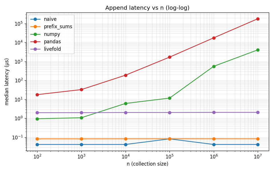
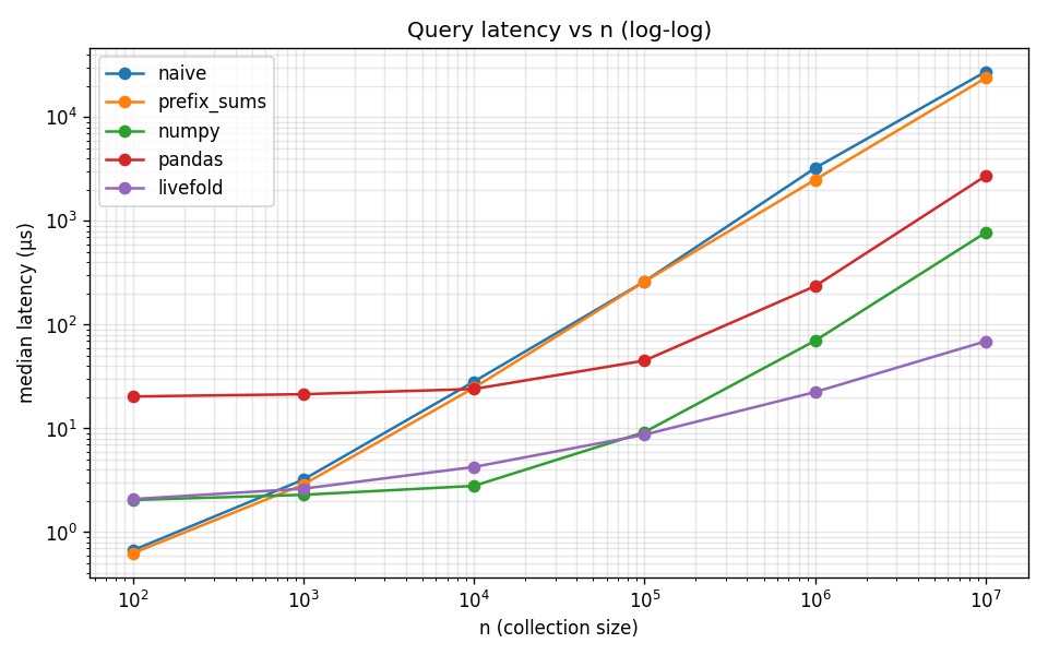
More details on the benchmark can be seen here.
Where it fits
The following table can be used to identify where livefold sits relative to other tools in the sequential range-aggregation toolbox:
Try it
If you have a mutable sequence and want exact range queries under any associative fold, livefold is on PyPI:
pip install livefoldAll code, benchmarks, and runnable Streamlit demos can be found here.